Kinematics of a Particle
Kinematics of a Particle
In this chapter, we analyze the motion of bodies without investigating its causes.
The Particle
To facilitate our observations of an object’s motion, we can describe the state of a body using spatial coordinates relative to a point. We call this point material point or particle. It is an idealized body in which all the mass is concentrated at a single point.
The Position Vector
To describe the position of a body at time \(t\) we use a coordinate system. In most cases, we will use a three-dimensional orthonormal coordinate system. The three coordinates \({x, y, z}\) therefore describe the position of the observed material point \(m\) (or, in the case of a rigid body, its center of mass). Along a certain path \(\Gamma\), the three coordinates will be functions of time:
\[\begin{equation} x(t),\; y(t),\; z(t) \end{equation}\]
We can now define the position vector \(\vb{r}(t)\):
\[\begin{equation} \vb{r}(t) := \begin{pmatrix} x(t)\\ y(t)\\ z(t) \end{pmatrix} \end{equation}\]
The position vector is defined with respect to the origin of the reference frame1 and therefore cannot be freely translated.
To calculate the length of a position vector, we use the following formula:
\[\begin{equation} r := |\vb{r}| = \sqrt{x^2 + y^2 + z^2} \end{equation}\]
For the direction of a position vector, we use the symbol \(\hat{\vb{r}}\):
\[\begin{equation} \vb{e_r} \equiv \hat{\vb{r}} := \frac{\vb{r}}{r} \end{equation}\]
This vector always has a length of 1.
The displacement vector gives the distance between the position at time \(t_1\) and time \(t_2\), that is, both the distance and the direction of the displacement of the material point (see Figure 1.1):
\[\begin{equation} \Delta\vb{r} = \vb{r}(t_2) - \vb{r}(t_1) \end{equation}\]
Conversely, the distance traveled along the curve \(\Gamma\) is given by:
\[\begin{equation} \int_{\Gamma}{\abs{d\vb{r}}} = \int_{\Gamma}{\sqrt{(dx)^2 + (dy)^2 +(dz)^2}} \end{equation}\]

Velocity
Velocity as a vector
Velocity \(\vb{v}\), like position, is also a vector; it indicates not only how fast we are moving but also in which direction. To calculate the average velocity \(\ev{\vb{v}}\), divide the displacement vector by the respective time interval:
\[\begin{equation} \ev{\vb{v}} := \frac{\Delta \vb{r}}{\Delta t} \end{equation}\]
Considering the limit as \(\Delta t \rightarrow 0\), we obtain the instantaneous velocity:
\[\begin{equation} \vb{v}(t) := \lim_{\Delta t \rightarrow 0} \frac{\vb{r}(t + \Delta t) - \vb{r}(t)}{\Delta t} = \dv{\vb{r}(t)}{t} = \dot{\vb{r}}(t) \end{equation}\]
To obtain the three components of the velocity vector, differentiate the three components of the position vector:
\[\begin{equation} \vb{v}(t) = \dot{\vb{r}}(t) = \begin{pmatrix} \dot{x}(t)\\ \dot{y}(t)\\ \dot{z}(t) \end{pmatrix} \end{equation}\]
Velocity is always tangent to the path.
Uniform Rectilinear Motion
As a first example, consider a body moving with constant velocity \(v_0\) along a straight line \(g\) passing through the origin of our reference frame. We choose the velocity such that it lies in the \(xz\) plane and is inclined at a certain angle \(\alpha\) with respect to the \(x\)-axis. The three velocity components are:
\[\begin{equation} \vb{v}(t) = \begin{pmatrix} v_x \\ v_y \\ v_z \end{pmatrix} = \begin{pmatrix} v_0 \ cos(\alpha)\\ 0 \\ v_0 \ sin(\alpha) \end{pmatrix} \end{equation}\]
Integrating the velocity components, we obtain the position vector:
\[\begin{equation} \vb{r}(t) = \begin{pmatrix} x(t)\\ y(t)\\ z(t) \end{pmatrix} = \begin{pmatrix} x_0 + v_0t \ cos(\alpha) \\ y_0 \\ z_0 + v_0t \ sin(\alpha) \end{pmatrix} \end{equation}\]
\(x_0, \ y_0\) and \(z_0\) are the constants of integration and represent the initial position of the body at time \(t_0 = 0\). We can choose the reference frame such that the body is located at the origin at time \(t_0\), to simplify calculations.
Acceleration
Acceleration as a vector
The acceleration \(\vb{a}\) is also a vector. Indeed, we are interested not only in how much we are accelerating, but also in which direction.
We define the average acceleration as the ratio of the change in velocity over a certain time interval:
\[\begin{equation} \ev{\vb{a}} := \frac{\Delta \vb{v}}{\Delta t} \end{equation}\]
Taking the limit as \(\Delta t \rightarrow 0\), we obtain the instantaneous acceleration:
\[\begin{equation} \vb{a}(t) := \lim_{\Delta t \rightarrow 0} \frac{\vb{v}(t+\Delta t) -\vb{v}(t)}{\Delta t} = \dv{\vb{v}(t)}{t} = \dot{\vb{v}}(t) \end{equation}\]
Acceleration is therefore the derivative of velocity and the second derivative of position:
\[\begin{equation} \vb{a}(t) = \dv{\vb{v}(t)}{t} = \dot{\vb{v}}(t) = \dv[2]{\vb{r}(t)}{t} = \Ddot{\vb{r}}(t) \end{equation}\]
Or written in vector form with its components:
\[\begin{equation} \vb{a}(t) = \begin{pmatrix} \dot{v}_x(t) \\ \dot{v}_y(t) \\ \dot{v}_z(t) \end{pmatrix} = \begin{pmatrix} \Ddot{x}(t) \\ \Ddot{y}(t) \\ \Ddot{z}(t) \end{pmatrix} \end{equation}\]
Acceleration can cause a change in both the magnitude and the direction of the velocity. This means that a motion in which the magnitude of the velocity is constant could still be accelerated if the direction of the velocity were not constant (example: circular motion).
Constant Acceleration (Uniformly Accelerated Motion)
In this case, we consider a motion in which both the magnitude and the direction of the acceleration are constant.
\[\begin{equation} \vb{a}(t) = const. \end{equation}\]
\[\begin{equation} \implies \vb{v}(t) = \vb{v}(t_0) + \vb{a}_0 \int_{t_0}^{t} dt' \end{equation}\]
\[\begin{equation} \implies \vb{v}(t) = \vb{v}_0 + \vb{a}_0 \Delta t \end{equation}\]
Similarly, we have:
\[\begin{equation} \vb{r}(t) = \vb{r}_0 + \vb{v}_0 \Delta t + \frac{1}{2} \vb{a}_0 (\Delta t)^2 \end{equation}\]
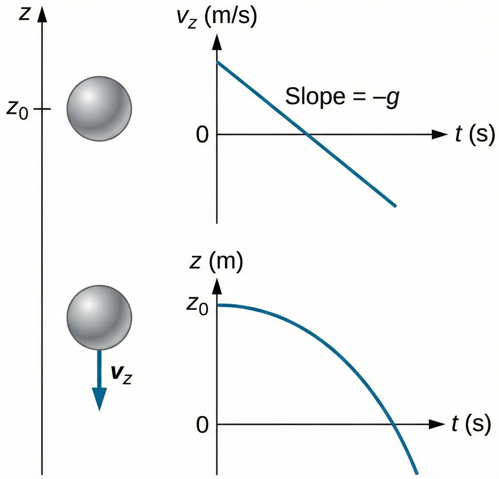
Example 1. Free fall
Consider an object in free fall and choose a reference frame in which the \(z\)-axis points upwards. Then the acceleration is:
\[\begin{equation} \vb{a}(t) = \begin{pmatrix} 0 \\ 0 \\ -g \end{pmatrix} \end{equation}\]
where \(g\) is the gravitational acceleration at the Earth’s surface and is equal to \(\SI{9.81}{\meter\per\second\squared}\).
Assuming the object has no initial velocity, we obtain the equation of motion for the body:
\[\begin{equation} \implies \vb{r}(t) = \begin{pmatrix} x_0\\ y_0\\ z_0 -\frac{1}{2}gt^2 \end{pmatrix} \end{equation}\]
Example 2. Parabolic motion
An object that is launched always follows a perfectly parabolic path (assuming it is not influenced by external factors). In this case, we can consider the components separately. As before, \(\vb{a}_0 = \vb{g}\). This time, we consider as initial conditions:
\[\begin{equation} \vb{r}(0) = \begin{pmatrix} 0\\ 0\\ z_0 \end{pmatrix}; \quad \vb{v}(0) = \begin{pmatrix} v_0cos(\alpha)\\ 0\\ v_0sin(\alpha) \end{pmatrix} \end{equation}\]
Since the acceleration is directed exclusively downward, by decomposing the motion into its various components, we observe that horizontally the body moves with uniform rectilinear motion, while vertically it moves with uniformly accelerated motion:
\[\begin{equation} \implies \vb{r}(t) = \begin{pmatrix} v_0tcos(\alpha)\\ 0\\ z_0 + v_0t -\frac{1}{2}gt^2 \end{pmatrix} \end{equation}\]
In this case, \(t\) acts as a parameter. We can eliminate \(t\) to obtain the equation of the parabolic trajectory \(z(x)\):
\[\begin{equation} t = \frac{x}{v_0cos(\alpha)} \end{equation}\]
\[\begin{equation} z(x) = z_0 + \frac{xsin(\alpha)}{cos(\alpha)}-\frac{g}{2}\frac{x^2}{v_0^2cos^2(\alpha)} \end{equation}\]
Circular Motion
Consider a particle moving uniformly on a circle of radius \(r\). We choose a reference frame whose origin coincides with the center of this circle, and such that the motion takes place in the \(xy\) plane. Using polar coordinates, we therefore have:
\[\begin{equation} \rho (t) = r \end{equation}\]
The angle \(\varphi\) varies with time and is given by:
\[\begin{equation} \varphi (t) = \varphi_0 + \omega t \end{equation}\]
where \(\varphi_0\) indicates the angle at time \(t=0\). \(\omega\) is the angular velocity, and in our case it is constant.
Now expressing the position vector in Cartesian coordinates, we obtain:
\[\begin{equation} \vb{r}(t) = r \begin{pmatrix} cos(\omega t + \varphi_0)\\ sin(\omega t + \varphi_0)\\ 0 \end{pmatrix} \end{equation}\]
Consequently, the velocity is given by:
\[\begin{equation} \vb{v}(t) = \dot{\vb{r}}(t) = r\omega \begin{pmatrix} -sin(\omega t + \varphi_0)\\ cos(\omega t + \varphi_0)\\ 0 \end{pmatrix} \end{equation}\]
The velocity vector is not constant. Its direction changes continuously, and is always perpendicular to the position vector.
In contrast, the magnitude of the velocity
\[\begin{equation} \abs{\vb{v}(t)} = v(t) = \sqrt{\dot{x}^2 + \dot{y}^2+\dot{z}^2} = r\omega \end{equation}\]
is constant.
We obtain acceleration differentiating once again:
\[\begin{equation} \vb{a}(t) = \dot{\vb{v}}(t) = -r\omega^2 \begin{pmatrix} cos(\omega t + \varphi_0)\\ sin(\omega t + \varphi_0)\\ 0 \end{pmatrix} = -\omega^2 \vb{r}(t) \end{equation}\]
We notice that the acceleration vector has the same line of action as the position vector but points in the opposite direction. This acceleration, always directed towards the center, is called centripetal acceleration. We also note that in circular motion with constant angular velocity, the magnitude of \(\vb{a}\) is constant over time. Despite this, the direction changes at every instant.
The magnitude of the centripetal acceleration depends on the distance from the center of rotation \(r\) and is proportional to the square of the angular velocity:
\[\begin{equation} a = r\omega^2 = \frac{v^2}{r} \end{equation}\]
Through the constant angular velocity, we can calculate the period of rotation of a body:
\[\begin{equation} T := \frac{2\pi}{\omega} = \frac{2\pi r}{v} \end{equation}\]
and the frequency of rotation:
\[\begin{equation} \nu := \frac{1}{T} = \frac{\omega}{2\pi} = \frac{v}{2\pi r} \end{equation}\]
The relationship between angular and linear velocity is therefore:
\[\begin{equation} \omega = \frac{v}{r} \end{equation}\]
Angular velocity as a vector
Consider now a circular motion taking place on a plane parallel to the \(xy\) plane at a distance \(z\). The magnitude of the velocity with respect to the center of the circle is:
\[\begin{equation} v = \rho \omega \end{equation}\]
We now define the angular velocity vector \(\vb{\omega}\), perpendicular to the plane of circular motion, obtaining the following equation:
\[\begin{equation} \vb{v} = \vb{\omega} \cross \vb{\rho} \end{equation}\]
Using a well-known vector identity we get:
\[\begin{equation} \vb{\omega} = \frac{1}{\rho^2}(\vb{\rho} \cross \vb{v}) \end{equation}\]
Angular Acceleration
In the case where the angular velocity is not constant, we define the angular acceleration as
\[\begin{equation} \alpha := \dot{\omega} = \Ddot{\varphi} \end{equation}\]
We now rewrite the position vector in the plane of rotation, assuming \(\varphi_0 = 0\):
\[\begin{equation} \vb{r}(t) = r \begin{pmatrix} cos\varphi(t)\\ sin\varphi(t) \end{pmatrix} \end{equation}\]
Velocity is then equal to:
\[\begin{equation} \vb{v}(t) = \dot{\vb{r}}(t) = r\dot{\varphi} \begin{pmatrix} -sin\varphi(t)\\ cos\varphi(t) \end{pmatrix} = r\omega \begin{pmatrix} -sin\varphi(t)\\ cos\varphi(t) \end{pmatrix} \end{equation}\]
The magnitude of velocity is given by:
\[\begin{equation} v = r{\omega}(t) \end{equation}\]
which is therefore no longer constant in time.
Linear acceleration is given by differentiating velocity in respect to time:
\[\begin{equation} \vb{a}(t) = \dot{\vb{v}}(t) = \underbrace{r\Ddot{\varphi}\begin{pmatrix} -sin\varphi(t)\\ cos\varphi(t) \end{pmatrix}}_{= a_{\parallel}} - \underbrace{r\dot{\varphi}^2\begin{pmatrix} cos\varphi(t)\\ sin\varphi(t) \end{pmatrix}}_{=a_{\perp}} \end{equation}\]
The acceleration is therefore expressed through two components. The first component is the tangential acceleration (\(a_{\parallel}\)), which is parallel to the linear velocity. The second component is the centripetal acceleration (\(a_{\perp}\)). The magnitudes of the two components are:
\[\begin{equation} \abs{\vb{a}_{\parallel}} = r \Ddot{\varphi} \end{equation}\]
\[\begin{equation} \abs{\vb{a}_{\perp}} = r\dot{\varphi}^2 \end{equation}\]
The coordinate system chosen for a physical problem is generally called a reference frame.↩︎